Buddhabrot

The Buddhabrot is an alternate visualisation of the Mandelbrot set, first described by Melinda Green and Lori Gardi. Warning: over 1MB in inline images on this page plus links to 10MB+ of high-resolution images.

Basic Method

The same iterative algorithm from the Mandelbrot & Julia sets is used, namely

Z_n+1 = Z_n² + C

Where Z and C are complex numbers. In the traditional Mandelbrot set, each pixel corresponds to a single constant C and the colour of the pixel is determined by the number of iterations before Z_n diverges (if at all) from a starting point of Z₀=0+0i. The Mandelbrot set is therefore a description of all Julia sets: the root orbit of each is a single point on the Mandelbrot set.

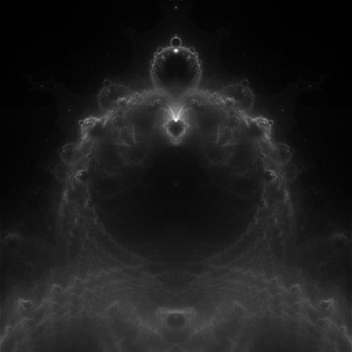
The Buddhabrot is a visualisation of the Mandelbrot set attractor - the paths taken by the iterations using constants C that result in divergence. This is calculated by filling a 2D histogram (1 bin per pixel) with the values taken by Z_n at each iteration step. Scaling this histogram to 8 bits (with a bit of overexposure) gives the following monochrome image:

To introduce colour, M. Green describes a technique whereby 3 histograms are maintained (1 per colour channel). For constant C resulting in divergence, the number of iterations taken to diverge is recorded and used to decide which histogram to increment with the iterations resulting from that constant. For example, with thresholds at 10², 10³ and 10⁴ for the R, G and B channels respectively:

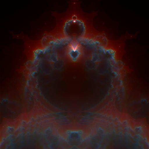
The fact that the image is no longer white indicates that the attractor followed by the Mandelbrot iteration is heavily dependent upon how long the iteration takes to diverge, i.e. constants with early divergence cause Z_n to follow a particular set of paths while constants that take longer to diverge take a different path through the complex plane. Areas of white in the image indicate heavy traffic - regions frequently traversed by iterations regardless of the divergence time.

The problem with these images is that they have little visible detail, a problem caused because some histogram bins are visited many more times than others. With only 8 bits of resolution per colour channel and linear scaling from histogram bin values to colour, much information is lost. Without over-exposure (loss of information in the high-traffic areas), much of the image remains black since the majority of histogram bins contain much less than 1/256th of the most full bins. Over-exposing brings out some of the detail in the dark areas, at the expense of information in the brighter areas.

New Transfer Functions

So, I experimented with alternate mappings from histogram values (X) to colours, namely exponential and logarithmic. The non-linearity introduced by these functions increases the "gain" for the more empty bins while reducing it for the more full bins. factor controls the degree of nonlinearity introduced.

f_lin(X) = X
f_exp(X) = 1 — e^{—factor * X}
f_log(X) = log(factor * X + 1)
scale = 255 * overexposure / f(X_max)
brightness(X) = scale * f(X)

The two images above (monochrome and colour) were taken using f = f_lin and overexposure = 2. For colour images, this calculation is performed 3 times, once per histogram / colour channel. The monotonicity of f ensures that max(f(X)) = f(X_max).

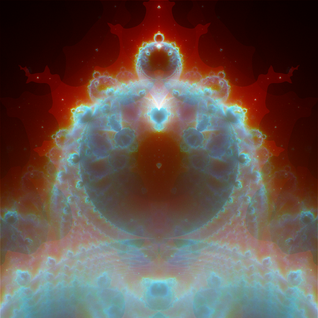
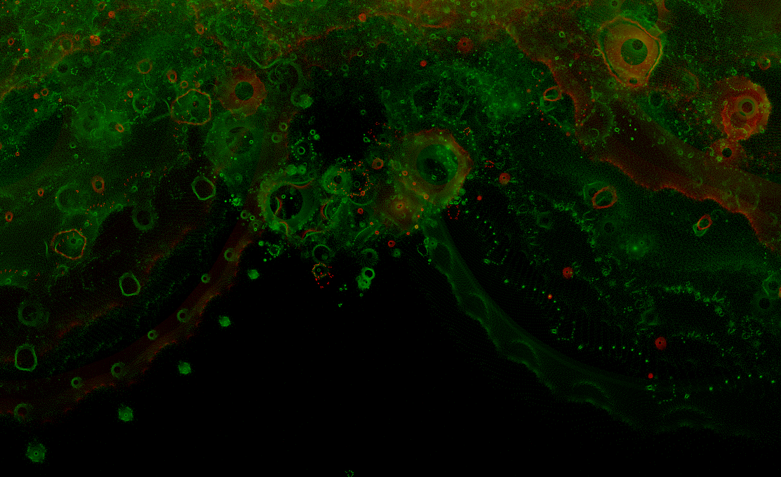
Now, the interesting images - note the dramatic increase in detail, particularly in the darker (lower traffic) areas. Each image links to a higher resolution, uncompressed version.

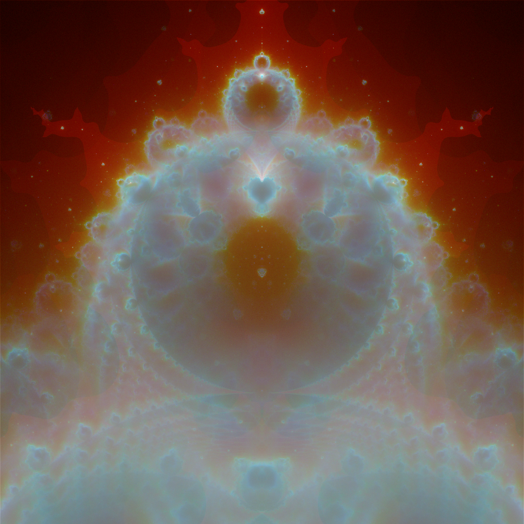
Each of the above was rendered with approximately 172*10⁶ orbits (different constants), for a total of approximately 888*10⁶ iterations. The above images are somewhat zoomed in, so each iteration does not necessarily fall within the domain of the histograms, therefore the total number of histogram hits is much smaller than the total number of iterations performed. This effect means that calculation becomes more computationally expensive the further the image is zoomed in: a smaller histogram domain means a smaller fraction of the iterations falling within that domain. Highly zoomed images require commensurately longer runtimes to accrue enough iterations within the histogram domain to provide an acceptable noise floor.

Long Iterations

The above images were created with relatively short iterations - orbits were abandoned on reaching 10⁴ iterations with the presumption that they lay inside the Mandelbrot set. These quickly-diverging orbits tend to have individual iterations well separated on the complex plane, thereby requiring many orbits before an acceptable noise floor is reached. Going beyond approximately 10⁸ orbits changes the image very little as it has converged to the attractor.

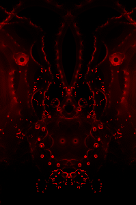
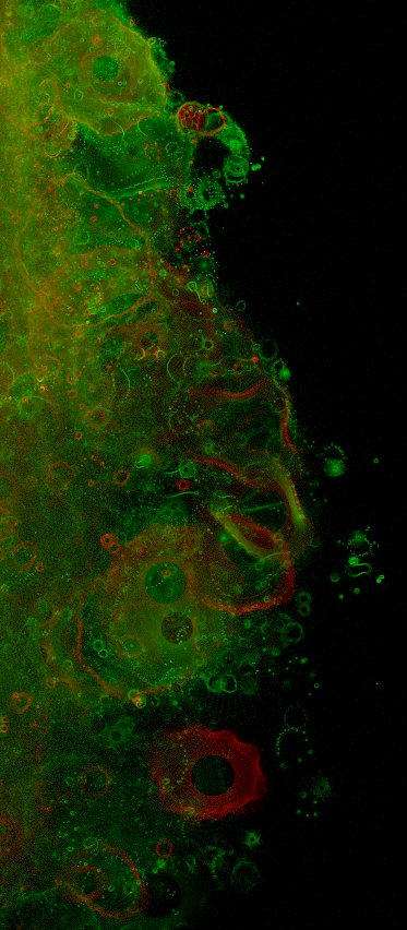
Use of longer iterations (10⁴ to 10⁶) yields an attractor in which the fine detail differs noticeably. The slower divergence means that individual iterations are often much closer together in the complex plane, thereby forming a distinct whorl, stroke, point or crenellation from each orbit. It is therefore no longer necessary to wait for a great many orbits to attain a "high quality" image - the variations introduced are quite beautiful in structure rather than noisy.

Increasing the number of orbits rendered tends to reduce the image to the same smooth attractor as seen with very few iterations; the fine structure becomes lost as the number of orbits approaches the millions and begins to average out the contents of the histogram.

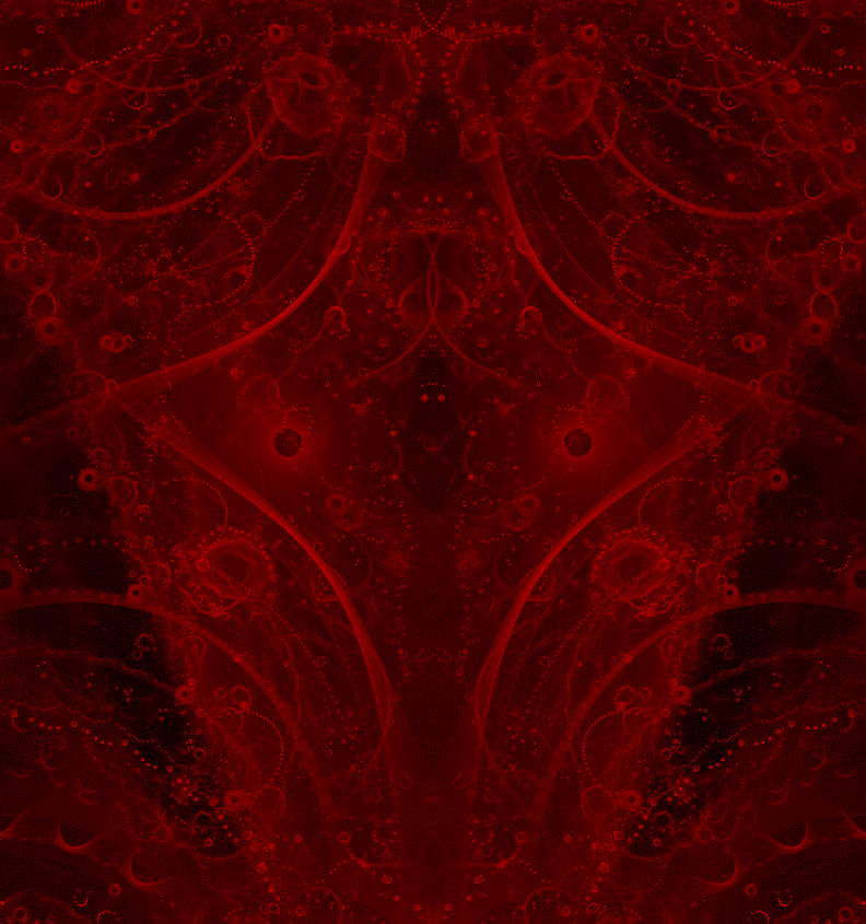
The following images are cropped from various parts of a 4096x4096 image of the whole buddhabrot.

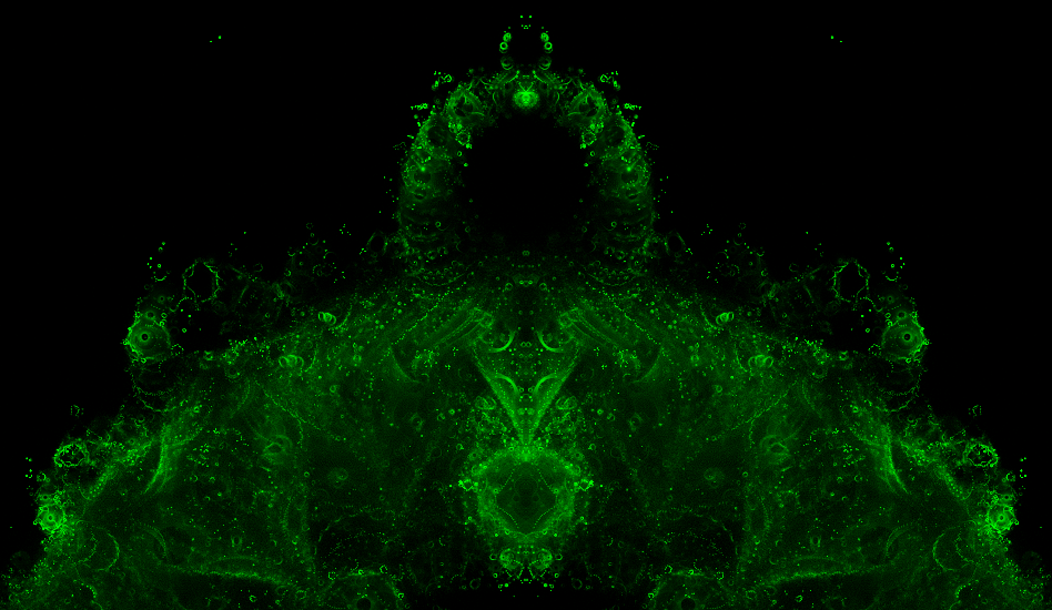
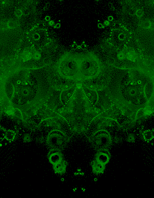
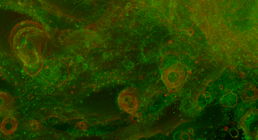
The images above are explicitly made symmetrical by adding the left & right halves of the histogram; without doing this the random order of appearance of the orbits becomes apparent, as below. The broad structure of the attractor (including its symmetry) is apparent, yet the fine detail is not subject to symmetry - each whorl is the result of a single orbit from a random constant C.

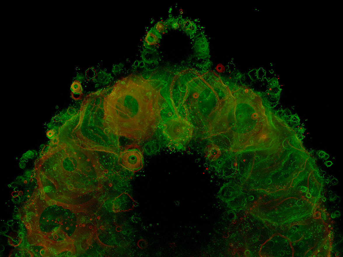
© 2004 William Brodie-Tyrrell. Last edit 2004-04-30.